Closed-Loop Design
From Basic Layer Information to Input-Output Characteristics
The following example demonstrates the predictive capabilities and accuracy
of the microscopic models used to set up the gain databases. It shows how
the databases can be used to predict fundamental operating characteristics
of operating devices using only basic information that is usually available
in an on-wafer stage of the development.
This example is outlined in more detail in Ref.[30]. Some
additional information about this example and general capabilities of the microscopic models
can be found in Ref.[35].
The structure is a ridge Fabry-Perot laser containing
of four 6nm wide In0.9Ga0.1As0.26P0.74/InP quantum wells.
The doping profile has been calculated to result in an internal electric
field across the active region of 80 kV/cm. The ridge is 3.8µm wide
and 750µm long.
From the reflectivities of the cleaved facets the outcoupling loss
is calculated to be 17.2/cm. Measurements of the threshold of devices of varying lengths
yielded an internal loss of 10.6/cm. The confinement factor is 0.0263.

Spontaneous Emission Analysis
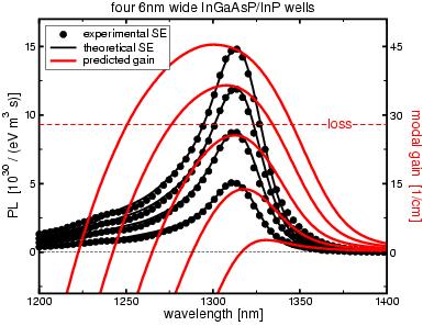
In
the first step the spontaneous emission (PL) of the un-processed sample
is measured for several excitation
densities in the low density regime. The results are shown as black dots in the picture above.
As described in the PL Analysis example and
Ref.[15], these spectra are compared to theoretical
ones in order to determine the inhomogeneous broadening (here: 14meV FWHM)
and possible deviations from the nominal structural design.
The theoretical spectra have to be shifted by -23nm corresponding to a slightly
smaller Indium- or Arsenic-concentration in the well than nominal.
The corresponding spontaneous emission spectra are shown as black lines in the picture above.
Also shown in that picture as red lines are theoretical gain spectra for several
carrier densities after applying the
determined inhomogeneous broadening and spectral shift.
Calculating Loss Currents
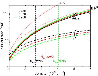
Using the fit-parameter free fully microscopic models described in detail in
Ref.[28] the loss currents due to radiative recombination
and Auger processes are calculated for various carrier densities.
the results are shown in the picture above for three temperatures.
Also shown in that picture as thin red lines are loss currents for 300K when using the power laws
BN² and CN³ for the radiative and Auger losses, respectively.
Here, the coefficients B and C have been determined from a fit to the microscopic results
at very low densities where the power laws are known to be fairly correct.
Despite knowing the correct low-density coefficients, these laws obviously overestimate dramatically
the loss currents in the density regime
relevant for laser operation.
The threshold carrier density, Nthr, is determined by looking up from the gain table
the density that yields enough gain after inhomogeneous broadening to overcome the outcoupling and internal
losses. The corresponding densities are marked by dashed vertical lines in the above picture.
Comparison to the Experiment
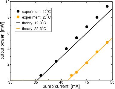
The picture above shows the experimental input-output characteristic
for this device at two temperatures (dots) together with what the theory would predict (lines).
The theoretical threshold is the sum of the Auger and radiative loss currents.
Defect recombination is assumed to be negligible in this high quality MBE-grown structure.
The slope of the characteristics is given by the ratio between outcoupling loss and total loss.
Assuming the nominal experimental tmperature the theoretical thresholds
are about 1.4mA too small. This slight mismatch is probably due to some
internal heating during operation. Assuming a 2.3K higher temperature than nominal
excellent agreement between theory is obtained.
It is worth stressing that these theoretical results do not include any adjustable
parameters. Of course, when using e.g. an Auger parameter, C, and its temperature
dependence as adjustable fit parameters, a good fit to experimental data
as shown here can easily achieved. However, such a fit requires previous knowledge of the
experimental result and has no predictive capabilities. Even trying to
extend the analysis by using the fitted Auger coefficients will generally fail
due to the sensitivity of the underlying processes to any variables like
temperature, density or structural variations.
In contrast, the only information used here is the nominal structural layout, the information about the
internal losses, the low excitation spontaneous emission spectra and general material
parameters from the standard literature.